experimental data acquisition
Prepare a sucrose solution with known concentration
and stabilize its temperature. Add an invertase solution to it and
simultaneously start the clock. Take samples of the reaction (discontinuous
assay) and transfer them, at precise times, to test tubes containing DNS (3,5‑dinitrosalicylic
acid). This stops the reaction in the samples by inactivating the enzyme and
also assays the reducing products, glucose and fructose, by measuring
absorbance at 540 nm. Repeat the procedure for several more sucrose
concentrations keeping the total enzyme concentration constant and low, but not
so low as to become saturated by the substrate. (Prepare a DNS absorbance standard curve in advance
using glucose standards.) model prescription
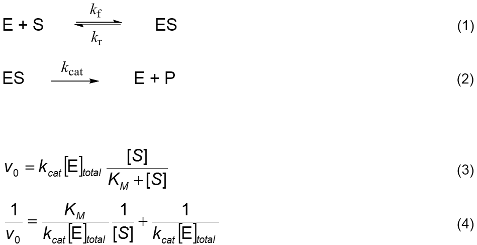
The Michaelis-Menten (MM) enzymatic process [1,2],
Reactions 1 and 2, is the simplest description of the action of a biological
catalyst. It considers the reversible formation of an enzyme-substrate complex,
ES, from which irreversibly results a product P. The overall process is S → P. The MM initial rate equation, Equation 3, is derived by assuming that
the process goes through a steady-state concentration of ES. It predicts that
the initial rate, v0, has
a limit when substrate concentration approaches infinity (catalytic sites
saturation), known as maximum rate: vmax
= kcat [E]total.
[E]total is the total enzyme concentration (or total catalytic sites
concentration) and KM is
the Michaelis‑Menten constant which can be expressed as (kcat + kr)/kf. Application of the MM rate equation is restricted to
conditions of negligible reverse rate of Reaction 2, that is, when product
concentration is zero or very low and/or the reverse rate constant of Reaction
2 is much lower than the forward rate constant (large equilibrium constant).
Rates should therefore be measured from time zero and using the smallest
possible time interval, starting with only substrate and enzyme. Generally,
product concentration will increase non-linearly with time but if a small assay
time interval is used, the length of which depends on the particular reaction
rate, the product increase will be apparently linear and the initial MM process
rate is easily obtained by linear regression, as illustrated in Figure 1. Non-linear regression of Equation 3 over {reaction
rate, [substrate]} data allows to estimate values for parameters KM and kcat at the experimental temperature. There are alternative linear rate functions for the MM
process. For example, the inversion of Equation 3 results in Equation 4, known
as Lineweaver-Burk’s. In this new arrangement, the linear variables are 1/v0 and 1/[S] and the linear
parameters are combinations of the original non-linear parameters: slope = KM/(kcat [E]total) intercept = 1/(kcat [E]total) Obtaining kcat
values at different temperatures is a means to estimate the activation entropy,
ΔS‡, enthalpy, ΔH‡, and Gibbs energy, ΔG‡, of the forward direction
of Reaction 2 by regression of the Eyring‑Polanyi equation [3], Equation
5, over {temperature, kcat}
data. In this equation, k is a rate
constant, kB is the
Boltzmann constant, h is the Planck
constant, R is the ideal gas constant
and T is temperature. It is derived
from transition state kinetic theory and can be linearized as Equation 6. Figure 2 summarizes all the experimental and
calculation procedures. computational function
Matlab files can be downloaded using the links at the
bottom of this page. Function kenz.m
is a simple implementation of the Matlab function nlinfit.m which estimates the parameters
of Equation 3 by nonlinear least squares fitting. Also, Matlab functions nlparci.m and ttest.m are used to
calculate, respectively, the uncertainty associated with the estimated
parameter values and the Student’s t-statistic for the residue sample against a
normal distribution of samples with mean zero. The code can be inspected with
any word processor and run in a Matlab console window using a command like: kenz(datavariablename, [kcat ,KM],
'namestring', o ) where datavariablename
is the name of a variable in the Matlab workspace containing values for the
experimental variables (see sample file below). The second argument of kenz.m is
a vector of initial values for the adjustable parameters (example:
[150 0.03]) and the last argument, o,
is set to 1 to perform regression or 0 to just plot data points and the
function curve calculated using the initial parameters. This last option is
useful to manually adjust the initial parameter values and see the effects on
the theoretical function. After a good initial parameter vector is found by
trial and error, the nonlinear fitting process is much more likely to converge. |
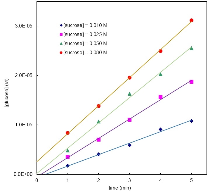
Figure
1 – The concentration of glucose increases in an apparently linear fashion as a
function of time, at least for the first five minutes. The linear regressions
do not extrapolate well to the origin, as it should, due to bad absorbance
reference setting by the students. However, the slopes are independent of that
setting and still give good estimates of the initial MM process rates. These
rates are used in Figure 3 (top). 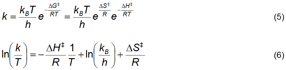
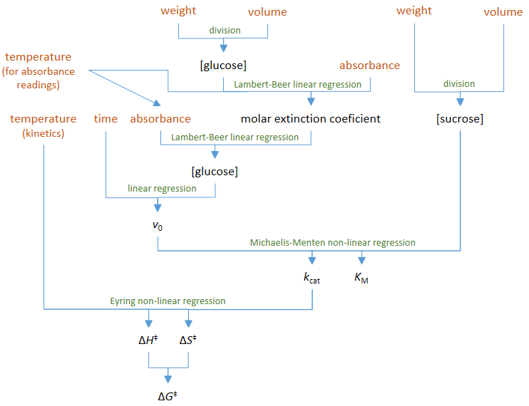
Figure
2 – Diagram summarizing experimental and calculation procedures. The
experimental measurements are coded with brown text and the calculations with
green text. Coded with black text are all the calculated quantities. 
|
examples and discussion
The enzyme invertase catalyses the almost
complete reaction of sucrose with water (hydrolysis) to produce glucose and
fructose, Reaction 7. This reaction is not formally similar to the theoretic MM
enzymatic process nor to the overall MM reaction S → P. But since water concentration is
essentially constant (it is the solvent), and the number of products is
irrelevant, because theoretically there is no reversal of reaction 2, it is
adequate to test the MM process description on invertase’s kinetic data with S
as sucrose.
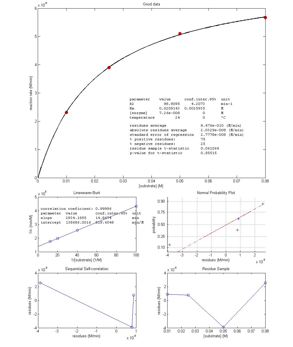
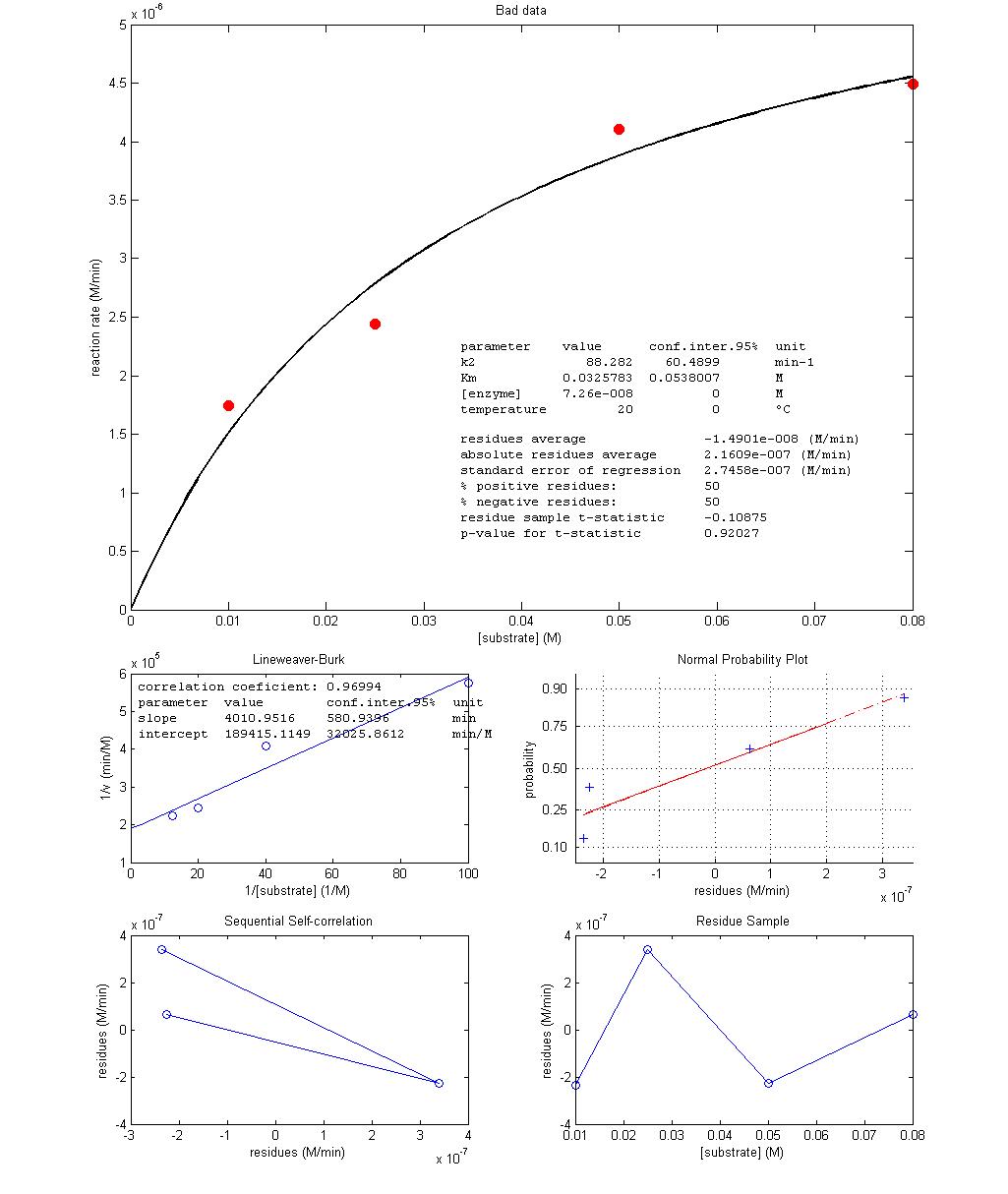
Figure 3 shows the best fit of Equation 3
over two experimental data sets obtained in class, one with low random errors
and another with high random errors. It is instructive to point out how
non-linear functions and its linearizations “interpret” noise differently. In
the low-error experiment, values obtained for kcat and KM by non-linear and linear regressions are
identical as expected (99/99 and 0.021/0.021, respectively) while in the
high-error experiment the two types of regression output very different values
(88/73 and 0.033/0.021, respectively). This means that 73/0.021 will not make a
good non-linear data fit while 88/0.033 will not make a good linear data fit
[4]. When noisy data is unavoidable then it all depends on the nature of the
noise sources. The reasonable option would be to go with the most natural
functional description of the target system, in this case the non-linear
function [5,6].
Notice that error estimates of linearized
functions parameter values also have to be correctly propagated to the original
parameters (slope and intercept to kcat and KM in this case) taking into account the
mathematical operations required for conversion.
It is also important to note that this
experiment is an accumulation of a series of interdependent procedures,
starting with the DNS/glucose absorbance standard curve and ending with the
Gibbs energy of activation (Figure 2). The best way to ensure low error on
parameter values, besides careful control and execution of procedures, is to
acquire the largest possible experimental data samples.
Figure
3 – Results from non-linear regression of Equation 3 with more precise (top)
and imprecise (bottom) experimental data.
|
references [1] https://en.wikipedia.org/wiki/Michaelis%E2%80%93Menten_kinetics (Jan-2017) [2] Johnson, K. A., Goody, R. S. (2011) The Original Michaelis
Constant: Translation of the 1913 Michaelis–Menten Paper. Biochemistry,
50, 8264-8269. DOI: 10.1021/bi201284u [3] https://en.wikipedia.org/wiki/Eyring_equation (Jan-2017) [4]
https://www.mathworks.com/help/stats/examples/pitfalls-in-fitting-nonlinear-models-by-transforming-to-linearity.html
(Jan-2017) [5] Lente, G., Fábián, I., Poë,
A. J. (2005) A common misconception about the Eyring
equation. New J. Chem., 29, 759-760. [6] Espenson, J. H., in Chemical Kinetics and
Reaction Mechanisms, McGraw-Hill, New York, 1995, 2nd edn.,
p. 158 |
| ||||
