experimental data aquisition
Solutions of precisely known
concentrations of (1) a diprotic aminoacid, (2) a strong acid (like
hydrochloric acid, HCl) and (3) a strong base (like sodium hydroxide, NaOH) are
prepared with deionized and, if possible, decarbonated water. Setup a typical
titration: the analyte is the diprotic aminoacid solution in a beaker, also
containing a magnetic stirrer and a calibrated pH electrode, and the titrant is
a strong base solution in a burette. If possible, an argon atmosphere over the
beaker helps prevent acidification of the analyte solution caused by
dissolution of atmospheric CO2. If necessary, and before any
addition of titrant, a precisely known volume of the strong acid is added
to the analyte solution such that it’s pH value drops (preferably) below the
value of the lowest pKa of
the diprotic acid, pKa1.
This intends to have most of the aminoacid in its diacid form so that titration
data are dependent on the pKa1 value. Step-wise addition of
strong base is then started, taking note of stabilized pH values and
corresponding titrant volumes, until pH is (preferably) above the
analyte's highest pKa. The
temperature is controlled, or at least carefully monitored and registered.
Results can be analysed by a number of commercial software packages and
computer learning environments [1] but it is more didactic to develop a
theoretical model from chemistry’s first principles and to write the
corresponding computational code for regression. model prescription
Table 1 shows the four
reaction equations that have to be considered in a weak diprotic acid titration
with strong base (MOH), starting from its diacid form, H2A. The
complete dissociation of the strong base MOH is assumed (infinite equilibrium
constant). MOH0 and H2A0 are the initial concentrations after mixing
a volume of titrant, Vtitrant,
concentration MOHtitrant,
with a volume of analyte, Vanalyte,
concentration H2Aanalyte. For each titrant
addition, the initial concentrations are given by equations 1 and 2. The
adjustable parameter v accounts for practical situations where, at the beginning of the titration, the titrant’s pH
is not entirely a consequence of the dissociation of pure H2A (discussed below). The reaction system in Table 1 can be
described at equilibrium, in water, by equations 3 to 7. Equations 3 and 4 are
for the acidity constants of the diprotic acid, equation 5 is for the
self-dissociation constant of water, equation 6 is a material balance and
equation 7 is a charge balance. This system can be solved by isolating z,
that is, the equilibrium concentration of H+, to yield the fourth
degree polynomial expressed in equation 8. Substitution of equations 1 and 2
into equation 8, and changing the variable z by the corresponding
chemical symbol, [H+]eq, results in equation 9. This
equation is hard to solve analytically for [H+]eq,
because it is a quartic
polynomial [2], but it is easily solved computationally by numeric
methods. Potentially, a fourth degree polynomial has as much as
four different roots but only one will be a real positive number
with physical meaning, given the constraints of the system. The
computational function that finds the roots of equation 9 has the form of
equation 10 where [H+]eq (the dependent variable), is a
function of Vtitrant (the independent variable) and of
parameters MOHtitrant, H2Aanalyte,
Vanalyte, Ka1, Ka2 and v.
Regression of equation 10 over an experimental data set {Vtitrant,
pH} estimates the values of the parameters H2Aanalyte,
Ka1 and Ka2, that is, the concentration of
the diprotic aminoacid and its acidity constants. The parameters MOHtitrant,
Vanalyte and Kw are known. The value of Kw
must be valid for the analyte's temperature and ionic strength. Volume v is an adjustable parameter
expressed as a titrant volume, for ease of interpretation, and it accounts for
the fact that the analyte solution may not be in the initial equilibrium state
presumed in Table 1. According to the defined chemical system, this state is a
consequence of producing the analyte by dissolving an amount of the pure diacid
species H2A in pure water, or any equivalent procedure. This means
that the initial pH of the analyte (before any addition of titrant) is described
as set only by H2A (and water) protolysis. If the actual titrant’s
initial equilibrium state is different from the one presumed in the chemical
description then the value of parameter v
compensates for it. For example, if one adds a volume of a strong acid, or a
strong base, to the analyte such that its pH becomes exactly equal to the one
obtained by the dissolution of pure H2A then regression over
titration data will estimate a value of zero for parameter v. If the initial pH is lower than that then v will have a positive value (more titrant needed) while if it’s
higher then v will be negative (less
titrant needed). The volume Vanalyte
is the volume at the start of the titration and must include all pre-titration
additions of strong acids or bases meant to set some actual initial equilibrium
state. computational function
Matlab files can be downloaded using the
links at the bottom of this page. These are simple implementations of the
Matlab function roots.m,
to find the roots of equation 9 and hence evaluate equation 10, and of Matlab
function nlinfit.m which estimates the parameters
of equation 10 by nonlinear least squares fitting. Also, the Matlab
functions nlparci.m and ttest.m are used to calculate,
respectively, the uncertainty associated with the estimated parameter values
and the Student-t statistic for the residue sample against a normal
distribution of samples with mean zero (the null hypothesis). The pot.m function plots the
experimental points and a line representation of the best fit of equation 10.
The code can be inspected with any word processor and run in the Matlab console
window with a command like: pot(datavariablename,
[H2Aanalyte, pKa1, pKa2,
v], 'namestring', o); where datavariablename is the name of a
variable in the Matlab workspace containing the titration data and the constant
parameter values (see sample file below). Using the correct value of Kw
is critical for fitting quality. This value is 1.0 x 10–14.0
for pure water, 1 atm and 298 K but it increases with temperature (pKw decreases) since water
ionization is endothermic (approx. +13 kcal mol–1 [3]). Kw also increases with ionic
strength I, from I = 0 to around I = 0.5
mol dm–3 and decreases for higher values of I [4]. The second argument of pot.m is a vector of initial
values for the adjustable parameters (example: [0.05 2.3 9.6 -1]). The string 'namestring' is used to identify the
plots, and the last argument, o,
should be set to 1 to perform regression or 0 to just plot the data points and
the function curve using the initial parameter values. This last option is
useful to manually adjust the values and see the effects on the theoretical
function. After a good initial vector is found by trial and error, the
nonlinear fitting process is much more likely to converge. |
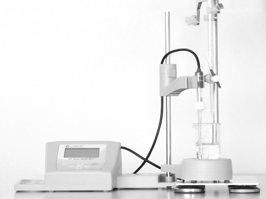
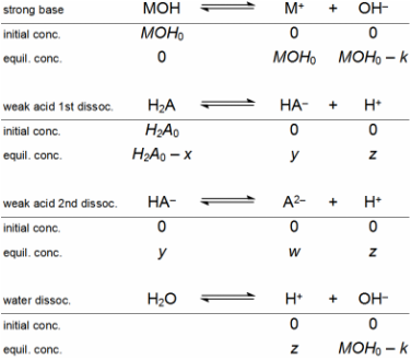

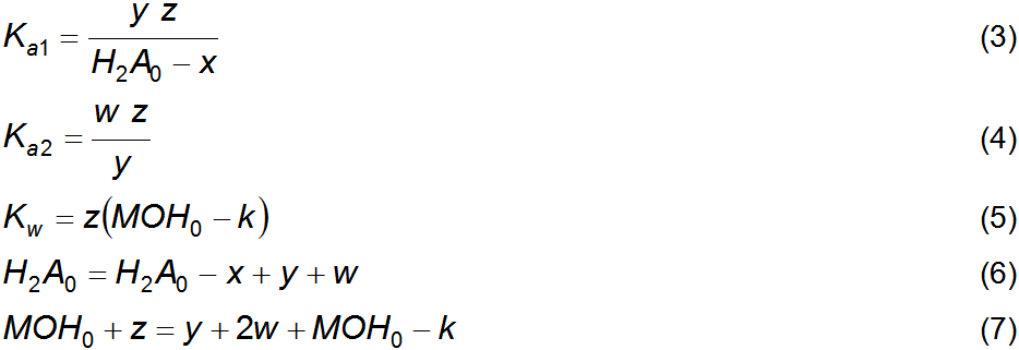


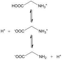
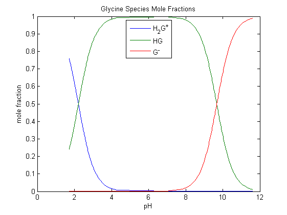
Figure 2 – Species distribution diagram for a glycine
titration (see Figure 3). |
examples
and discussion
Glycine is diprotic and mainly in its diacid form at low pH values
(Figure 1). The glycine analyte solution was prepared
originally as 50 cm3 of 0.050 mol dm–3 glycine, HOOC–CH2–NH2,
which has a pH value near 6. A volume of 2.5 cm3
of HCl 1 mol dm–3 (equimolar) is added to that solution to lower its pH value to the value
it would have if pure diacid glycine were dissolved.
Figure 2 is a species distribution diagram taken from one of the example
titrations discussed below and it shows how glycine’s carboxylic acid group is substantially dissociated at the beginning of the
titration. However, since all the free H+ derives stoichiometrically from that group then the expected value
of Vequiv
for its exact titration is 10.0 cm3 with NaOH
0.25 mol dm–3.
The same volume is necessary to exactly titrate the
ammonium group.
Figure 3 shows
three examples of student-made potentiometric titrations of glycine with NaOH 0.25 mol dm–3
and the results of nonlinear regression of equation 10 over the acquired data.
A value of 13.8 for pKw
was used based on temperature and ionic strength
experimental conditions [4]. Vequiv can be estimated
from experimental results in two ways: Vequiv = Vendpoint1
– v = Vendpoint2 – Vendpoint1.
The regression value of parameter v
for Titration 1 shows that a fair excess of HCl was
accidentally added to the titrant solution while in the other two experiments
the opposite occurred The fit seem quite good, despite
no decarbonated water, temperature control or inert
atmosphere were used. The Residue Sample plots show slight, non-random, wavy
trends along the titrations, with a non-random spike near endpoint 1. However,
this deterministic trend is very small when compared with data variation. p-values,
Sequential Self-correlation plots and Normal Probability plots all agree that
the most random residue sample is that of Titration 2 and the least random
comes from Titration 3. However, Titration 3 becomes much better than the other
two if a value of 13.6, instead of 13.8, is used for pKw.
While the higher pKw
“informs” regression that water is more acidic this is not experimentally
justifiable since Titration 3 was performed at a lower temperature and
therefore pKw
for this experiment should be higher than 13.8, not lower. Better fitting with
lower pKw
may be explained as compensating the carbonation of the titrant, not included
in the description of the target, which leads to excessive acidity caused by
aqueous CO2 (carbonic acid, pKa1
= 6.3) and HCO3– (pKa2
= 10.3). This explanation can be validated by
repeating the titration with decarbonated solutions
under an argon atmosphere and/or less vigorous titrant stirring.
With few exceptions, like that of
Titration 3, experimental data validate the applied model. Besides carbonation,
other causes of error are debated with the students,
such as taking pH readings before value stabilization, temperature drifts, the
use of concentrations instead of activities and less than good pH electrode
performance outside the calibration buffers pH range. The uncertainty estimates
of the parameters are assessed as acceptable and the
relation of that uncertainty with the number of points fitted is made by
repeating the regression with fewer experimental points. The regression
estimates of glycine’s acidity constants are compared
with expected values, and relative errors are calculated.
Other methods of obtaining the glycine titration parameters from the
same data sets are discussed and compared, namely, the
use of the Henderson-Hasselbalch equation (equation 11). The point is made that
estimation of pKa1 and pKa2 values by data
interpolation relies heavily on equivalence volume estimation an this, if at all possible by non-regression methods, is
always more rigorous if some continuous function is fitted to the experimental points
[5].
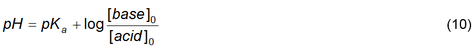
Figure 3 – Three
potentiometric titration plots of fully protonated glycine (
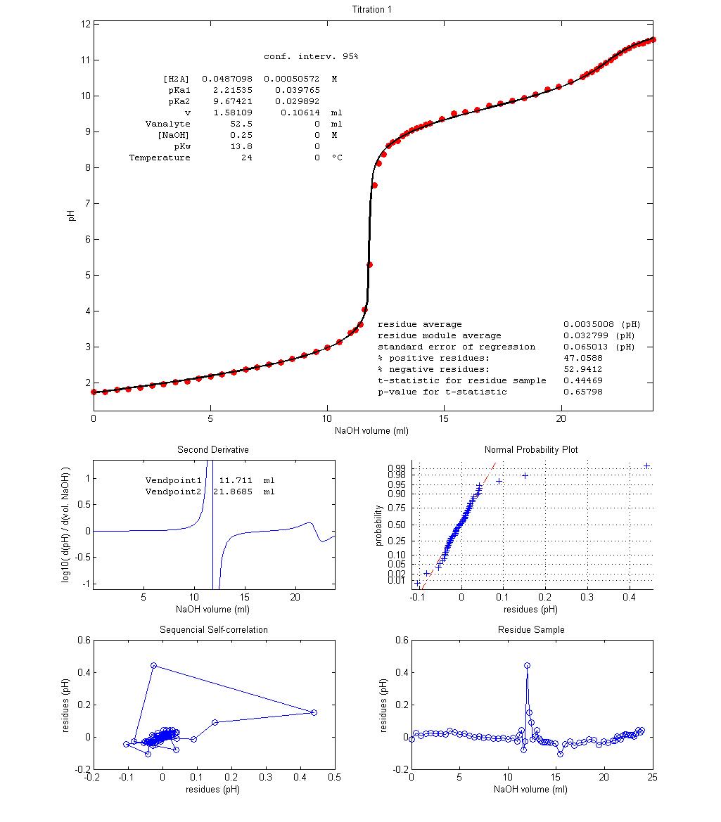
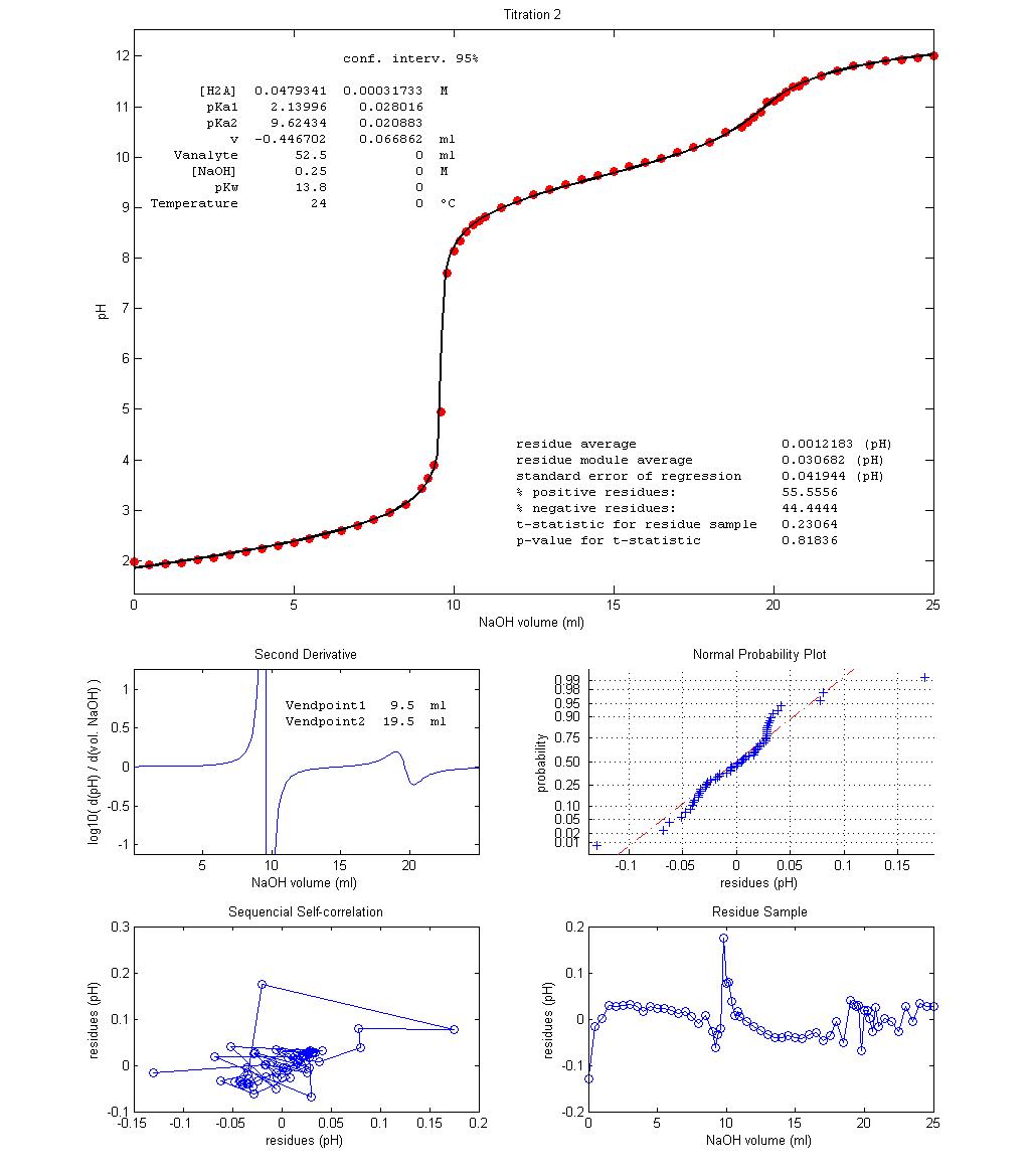
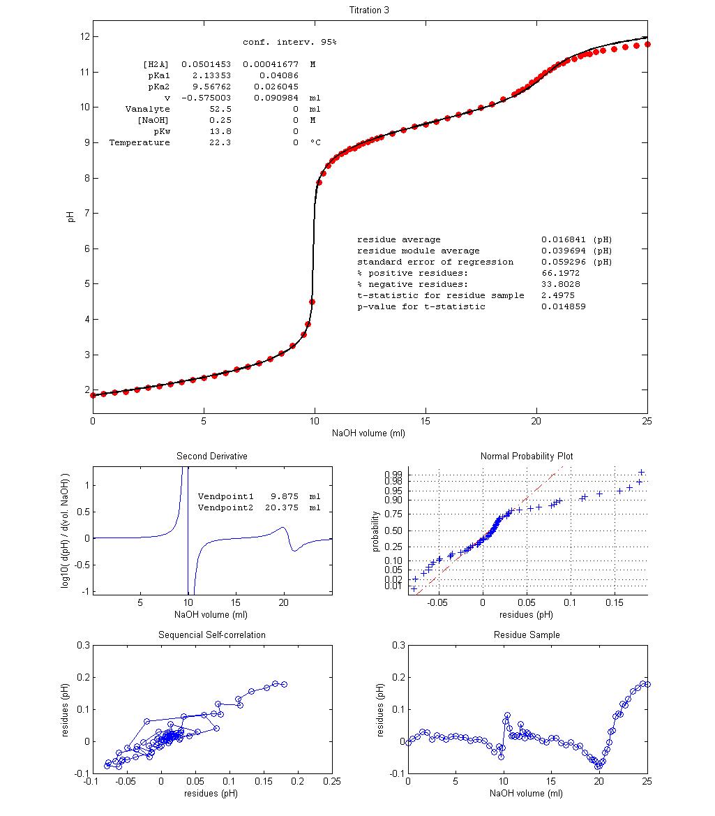
|
references [1]
Heck, A, Kędzierska, E, [2] http://en.wikipedia.org/wiki/Quartic_function. [3] Cerruti,
PJ, Ko, HC, McCurdy, KG, Hepler, LG (1978). The
standard enthalpy of ionization of water at 298 K from calorimetric
measurements on iodine pentoxide. Canadian Journal of Chemistry, 56, 3084–3086. [4] Vilariño,
T, Sastre de Vicente, ME (1997). Theoretical calculations of the ionic strength dependence
of the ionic product of water based on a mean spherical approximation. Journal of Solution Chemistry, 26, 833-846. [5]
Ma, N.L., Tsang, C.W. (1998). Curve-Fitting Approach to Potentiometric
Titration Using Spreadsheet, Journal of Chemical Education, 75, 122-123. |
| ||||
